Little-studied man-made gases have big warming potential

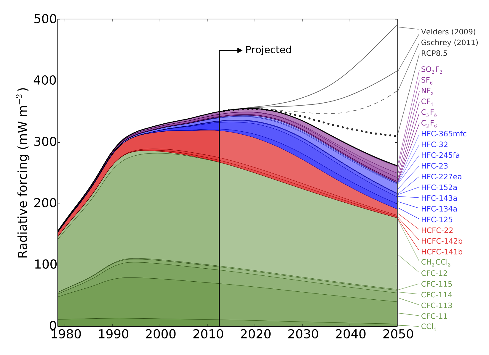
We recently published a paper “Recent and Future Trends in Synthetic Greenhouse Gases” in Geophysical Research Letters describing recent trends in “synthetic” greenhouse gases (gases with no significant natural sources), and their possible impact on climate in the coming decades. The paper was summarised on the American Geophysical Union blog (thanks to Alexandra Branscombe!), and is described in the following University of Bristol press release:

Radiative forcing due to synthetic greenhouse gases. Historical values are based on AGAGE observations. Future values assume the HFC phase down schedule proposed by the US Environmental Protection Agency (2012), compared to previously published "non-policy" scenarios.
Radiative forcing due to synthetic greenhouse gases. Historical values are based on AGAGE observations. Future values assume the HFC phase down schedule proposed by the US Environmental Protection Agency (2012), compared to previously published “non-policy” scenarios.

The total warming impact of 25 major synthetic greenhouse gases has been examined by an international team, led by researchers from the University of Bristol.

The study estimates that, without additional limits on synthetic greenhouse gas use, the resulting increase in warming could outweigh the climate benefits gained thus far from phasing down chlorofluorocarbons (CFCs).

CFCs—commonly used in refrigerators and air conditioners—garnered public attention for their role in creating a hole in the ozone layer over Antarctica.  As these chemicals were phased-down thanks to international agreements limiting their use, they were replaced by other synthesized gases that can still be harmful to the ozone layer and are greenhouse gases that contribute to climate change.  Despite this, synthetic greenhouse gases (SGHGs) beyond the CFCs have received relatively little attention from the research community—until now. 

The study, led by Dr Matthew Rigby in Bristol’s School of Chemistry, analysed observed atmospheric levels of SGHGs from 1978 to 2012, and then used these measurements to predict the impact these gases could have on global warming through 2050.

In response to the phase-down of CFCs through the 1987 Montreal Protocol, the researchers discovered that the use of other synthetic gases as refrigerants—such as hydrofluorocarbons (HFCs)—has risen.  HFCs had been limited in the now-defunct 1997 Kyoto Protocol, but there is currently no agreement restricting their use.  So, using HFCs as a test case, the researchers examined the effect of phasing down HFCs by amending the Montreal Protocol to include these gases.

Dr Rigby said: “We could avoid adding the equivalent of up to another three years of carbon dioxide emissions into the atmosphere if these gases were being phased down.”

HFCs are particularly strong greenhouse gases, so even relatively small levels in the atmosphere can contribute to warming.

“Per tonne of emissions, HFCs are much more potent greenhouse gases than carbon dioxide, and are very good at trapping the radiation that heats the Earth,” Dr Rigby said.

While HFCs are currently not a major driver of climate change compared to carbon dioxide or even other SGHGs, the researchers point out that if unabated they may contribute significantly to future warming.

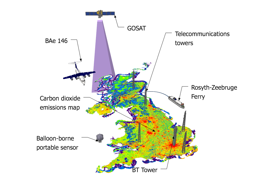
The study used measurements of SGHG levels from the Advanced Global Atmospheric Gases Experiment (AGAGE), a global observing system developed by Professor Ronald Prinn of the Massachusetts Institute of Technology (MIT) and colleagues, and sponsored by NASA and other agencies.

Professor Prinn, co-director of the MIT Joint Program on the Science and Policy of Global Change and a co-author of the report said: “Addressing HFCs, and other SGHGs, now will ensure that they don’t contribute significantly to warming in the future.”

Meanwhile, the researchers note that due to extensive use, CFCs will continue to warm the planet for years to come.

“CFCs have contributed the most among the synthetic greenhouse gases to warming.  Their use peaked and levels are now declining, but these gases will remain in the atmosphere for many years.  This is likely the trend we will see with most SGHG gases, so it is important that we address these gases now before they do more severe damage,” said Professor Prinn.

(With particular thanks to Audrey Resutek who wrote the MIT press release that this is based on).

GAUGE kicks off!

GAUGE schematic

On the 1st March, we officially began our new £3m NERC-funded consortium project Greenhouse gAs Uk and Global Emissions (GAUGE). The University of Bristol press release explains:

Scientists awarded grant to determine UK’s greenhouse gas emissions
Press release issued 1 March 2013

Researchers in the University of Bristol’s Atmospheric Chemistry Research Group (ACRG), in collaboration with scientists around the country, have been awarded funding from the Natural Environment Research Council (NERC) to provide an independent ‘top-down’ check on the UK’s greenhouse gas emissions estimates.

GAUGE schematic
GAUGE will involve measurements of greenhouse gases from the air, sea and space in an effort to better quantify UK emissions

The UK is required to estimate how much climate-warming carbon dioxide, methane and nitrous oxide it emits each year. However, at the moment, these estimates rely heavily on so-called ‘bottom-up’ accounting methods that may be subject to biases and inaccuracies.

The GAUGE project (Greenhouse gAs Uk and Global Emissions) is a three and a half year collaboration between several universities and research institutions across the UK.

ACRG’s Professor Simon O’Doherty, who also runs the UK greenhouse gas monitoring network funded by the Department for Energy and Climate Change, said: “It’s important that we expand our greenhouse gas observation capabilities in this country, if we’re really going to understand what we’re emitting. But it’s equally important that we begin exploring new types of measurement, which may help us understand emissions processes more fundamentally.”

GAUGE will bring together a more comprehensive suite of greenhouse gas observations around the UK than has ever been compiled. The project will determine emissions using information from satellites, aircraft, tall towers (including the BT tower in the middle of London), balloons and boats.

In addition to developing new measurements, GAUGE will use computer models to simulate how greenhouse gases travel through the air.

Dr Matt Rigby, a research fellow at ACRG, said: “By measuring the concentration of greenhouse gases in the atmosphere, and then using computer models to simulate where the air came from in the days before the measurements, we can determine emissions from the surrounding areas. This new funding will allow us to develop these methods with the help of the Met Office and GAUGE partners at other universities.”

Using the new measurements and modelling techniques, GAUGE researchers hope to make the UK’s emissions amongst the best-quantified in the world.

Using new measurement technology to estimate methane sources

Delta-13C-CH4
MOZART simulation of 13C-CH4 in the atmosphere. The blue areas show parts of the atmosphere with a smaller fraction of the 13C-CH4 isotope than the atmospheric average, due to near-by emissions from microbial sources. In contrast, the red areas show air that is enriched in 13C-CH4, probably due to biomass burning.

Although methane is the second most important greenhouse gas its sources are quite poorly understood. However, new methods of measuring atmospheric methane may be able to help.

Methane is a molecule containing one carbon and four hydrogen atoms. These atoms usually have an atomic mass unit of 12 (carbon) and 1 (hydrogen). However, they also occur in higher masses in nature, called isotopes. Carbon-13 and deuterium (hydrogen with a mass of 2) occur in one atom for every few thousand atoms of regular carbon or hydrogen. This becomes potentially useful for us, because different sources of methane emit molecules with slightly different ratios of carbon-12 to carbon-13 or different ratios of hydrogen to deuterium. For example, methane emitted from wetlands has less 13C than the average in the atmosphere, whereas wildfires emit methane with a relatively high deuterium content.

So, by measuring methane concentrations and isotope ratios in the atmosphere, we can hope to learn something more about where the methane came from.

In the last few years, advances in laser spectroscopy have meant that we can now measure the isotopic composition of methane by shining lasers through a sample and measuring the absorption of certain wavelengths. However, the variations in methane isotope ratio that we expect to see in the atmosphere are very small. Therefore, to be able to resolve small changes, some people are proposing to also “pre-concentrate” air samples, which means that we remove a lot of the nitrogen, oxygen and other major components of air, to leave a more concentrated sample of methane that can be analyzed. Similar systems exist for measuring concentrations of other gases, but not yet for methane isotopes.

In this paper, we asked the question: “If we had these instruments at each AGAGE station, how much better would we be able to constrain methane emissions from different sources than we can at present?”. The answer we found was a little mixed. We found that these new measurements would provide additional information about the methane emissions to the atmosphere. However, the amount by which the uncertainties in our current estimates of methane emissions would be reduced is a little smaller than we hoped for. For example, for wetlands (the single largest source) and other microbial sources, we found that global uncertainty reduction would be reduced by only around 3%. For smaller sources that had a more “distinct” source isotope ratio such as biomass burning, larger relative uncertainty reductions were possible (9%).

Despite the relatively modest uncertainty reductions, my feeling is that, given the importance of methane in the global climate system, these new instruments will have a role to play in a future methane observing system. Given the complexity of the system, no single measurement (or modeling) strategy will be able to fully determine the causes of the strange changes we see in methane. However, by combining many measurement types, we should be able to understand the system better than we currently do.

Combining two models for emissions estimation

In the AGAGE network, we have a small number of monitoring stations, which measure greenhouse gases at high frequency. I’m interested in using these high-frequency measurements to estimate emissions from the countries surrounding the sites.  To connect the measurements to sources, we require chemical transport models (see some animations here). However, when we use global models, they take a lot of computer time to run, particularly at high resolution, which is needed when we’re trying to estimate emissions on national scales.  Sometimes it makes sense to run a model at very high resolution close to the measurement sites (where we have the most information about emissions) and low resolution everywhere else.  This was the problem we tried to tackle in this paper, co-written by colleagues at the UK Met. Office.

The method we developed takes the output from two different types of model and couples them together so that we could estimate emissions at very high resolution close to the monitoring sites, and low resolution further away.

Average 'footprints' around four AGAGE monitoring sites. Generated by the UK Met. Office NAME model.

We’ve used this method, along with the the Met Office NAME model and NCAR’s MOZART model, to determine SF6 emissions around four AGAGE sites (see the figure), and will be extending it to all the other AGAGE gases in the near future.

The code for the project can be found at Google code: http://code.google.com/p/mr-cels/

Four new HFCs

Hydrofluorocarbons (HFCs) are replacements for chlorofluorocarbons (CFCs), whose use is being phased out because they are primarily responsible for depleting the ozone layer. While HFCs don’t destroy ozone, they are often very powerful greenhouse gases, so it is important that we monitor their concentration and emissions. One difficulty in doing this is that there are many HFCs emitted into the atmosphere, and new ones are appearing all the time.

To keep track of these gases, my colleagues in the AGAGE network have developed a system that can measure gas concentrations using mass spectrometry. The system is able to detect gases at very low concentrations, by removing most of the nitrogen and oxygen from the measured samples, increasing the concentration of the pollutants they want to measure. This means that we can now detect ‘new’ gases very soon after they appear in the atmosphere.

In this paper, Martin Vollmer from Empa in Switzerland describes the measurement of four HFCs that have appeared in the atmosphere over he last decade or so (HFC-227ea, HFC-236fa, HFC-245fa, HFC-365mfc). Using a combination of in situ measurements, and new measurements of archived air samples, we can determine the entire air history of the four gases, from the year they first appeared in detectable amounts.

Measured mixing ratios of four new HFCs

Using these observations, and a two-dimensional model of the atmosphere, we calculated the annual global emission rates. As is often the case, the emissions we found differed from inventory estimates by substantial amounts, highlighting the value of these sort of ‘top-down’ verification techniques.

Deriving emissions time series from sparse observations

Over the last couple of years, a few of us at MIT and Scripps have been thinking about how we could estimate trace gas emissions over several decades using archived air samples.  For example, the Cape Grim Air Archive, from Tasmania, is a really nice collection of air samples that have been taken under carefully controlled conditions over many decades.  The archive was set up so that as measurement techniques improved, we could monitor the history of important atmospheric gases that were difficult to measure in the past.  We’ve used these observations to determine global emissions of species like the perfluorocarbons (see Jens Muhle’s paper), and some newly-observed HFCs (in Martin Vollmer’s recent paper), all of which are very potent greenhouse gases.

However, one problem that we kept encountering was that, using our usual methods for determining emissions, we would get large ‘jumps’ in our derived emission, which we knew were unlikely to have occurred in the real world.  These fluctuations were probably caused by slight biases in the observations, or inaccuracies in the independent emissions inventories that we have to use as a first guess.  To get around this problem, we tried to think about how we could derive emissions using information on how we would expect emissions to change from one year to the next.  For example, if a gas is emitted by Aluminium smelters, then emissions are not very likely to change by more than a few percent per year, because the number of smelters, or the emissions processes, are unlikely to change very fast.

We found some techniques that addressed similar problems in other fields (notably Oceanography), and modified them so that they could easily be applied to atmospheric trace gas emissions estimation.  The result is a method that firstly allows you to estimate the emissions growth rate, based on some prior information, and the uncertainty that you expect this estimate to have.  Then a chemical transport model is used to produce an emissions estimate that best matches both the measurements, and our emissions growth constraint.  The paper, written with Anita Ganesan and Ron Prinn, can be found here.

Measurements of C3F8, a powerful greenhouse gas that stays in the atmosphere for thousands of years. Emissions derived using these observations and a growth-based estimation scheme are shown in the bottom panel.

History of Atmospheric SF6

Sulfur hexafluoride (SF6) is a particularly potent greenhouse gas.  It is used in large electrical equipment, and leaks into the atmosphere during maintenance.  Once it is in the atmosphere, it is only destroyed if it reaches very high altitudes, making it last for hundreds to thousands of years.  It is also a very strong absorber of infra-red radiation.  These factors result in it being one of the most potent greenhouses yet discovered.  One tonne of emissions is thought to be equivalent to releasing over 22,000 tonnes of CO2.

Global SF6 emission rate from 1970 to 2008. The solid line shows the estimate using AGAGE measurements.

In collaboration with many of my AGAGE and NOAA colleagues, we examined how concentrations of this gas have increased in the atmosphere since the 1970s, and determined global and regional emissions (see Atmospheric Chemistry and Physics paper).  We find that concentrations of SF6 have increased by more than a factor of 10 since our first measurement in 1973.  We also find that global emissions are now higher than ever, and have increased by almost 50% in the last 5-10 years.

We wanted to find out where this increase in emissions was originating from.  To do this, we used measurements made by the AGAGE and NOAA monitoring networks and a three-dimensional chemical transport model.  The model (called MOZART, developed by the National Center for Atmospheric Research), uses wind speeds and other meteorological information that have been calculated using weather forecasting models, to simulate how pollutants are transported around the world.  By testing how this model responds to changes in emissions from different regions, we can use the measurements to find out where SF6 originated from.

There were two major findings from our work.  Firstly, we find that it is very likely that all of the recent emissions increase is being driven by an increase in emissions from Asian countries that do not report detailed emissions to the United Nations Framework Convention on Climate Change (UNFCCC), such as China, India and South Korea.  Secondly, we find that developed countries that do report emissions to the UNFCCC (e.g. USA, UK, Germany), are likely to be underestimating their emissions.

Downloads

EDGAR emissions interpolated to 5×5 degrees and scaled in each hemisphere using AGAGE measurements between 1970 – 2008 can be found here in NetCDF format.

Regionally optimized EDGAR emissions at 1.8×1.8 degrees for 2004-2005 and 2006-2008 can be found here in NetCDF format.

Optimized 3D mole fraction fields at 5×5 degrees, and 28 vertical (sigma) levels are here in NetCDF format (10MB).

Renewed Growth of Atmospheric Methane

Methane is a strong greenhouse gas, and plays an important role in the chemistry of the atmosphere.  Global concentrations are currently more than double their pre-industrial values (as shown by ice core data).  However, in recent years this dramatic growth has slowed, and was close to zero between 1999 and 2006 (see graph below).

In this paper, published in Geophysical Research Letters, we presented AGAGE and CSIRO data showing renewed global growth of methane concentrations starting in 2007.  We speculated that some natural process was most likely responsible for such a rapid change in concentration, since anthropogenic emissions tend to change more slowly (a few percent per year).  For example, wetlands, the single largest source of methane, could have increased their emission rates in response to changes in temperature and precipitation (2007 was an extremely warm year over Siberian wetlands).  Alternatively, we note that a modest decrease in the concentration of the chemical that destroys methane, the hydroxyl radical (OH), could produce a sudden growth.

Methane mixing ratios at five AGAGE sites from 1997 to 2009. Annual mean growth rates are shown in the lower panel. Modified from Rigby et al., 2008.

There was an additional puzzle to this methane increase, which was that growth occurred across the globe at almost the same rate. Most of the methane sources are in the Northern hemisphere, so we would usually expect to see growth beginning in the North, and then propagating to the South later on.  This near-simultaneous rise in concentration in both hemispheres suggested that tropical emissions could have played an important role.

In the two years since the publication of this paper, lots of groups have examined these strange fluctuations in methane levels.  In particular, Ed Dlugokencky at NOAA and Philippe Bousquet at LSCE in France have written some very nice papers on the subject (Dlugokencky et al, 2009 in Geophysical Research letters and Bousquet et al, 2010 in Atmospheric Chemistry and Physics Discussions).  They find that the most likely explanation for the rise since 2007 has been an increase in emissions from northern wetlands in 2007 and then an increase in tropical wetland emissions in 2007-2008.  They find little evidence for a large change in OH concentration or large increases in biomass burning.

Our paper received some press attention in 2008 (e.g. MIT press release, “Climate Warming methane levels rose fast in 2007”, Reuters).  It was also quoted in several articles suggesting that melting arctic permafrost could be driving the increase (e.g. “A sleeping giant?”, Nature Reports Climate Change). How much the arctic permafrost melt is contributing to changing methane concentrations is still the subject of much research.  However, as mentioned above, it seems most likely that the recent increases can be explained by changes in output from existing wetlands.

In addition to these articles, the paper also caught the attention of some people who drew slightly unusual conclusions from the work.  Some thought we had “inadvertently disproved global warming” (“MIT Scientists Baffled by Global Warming Theory, Contradicts Scientific Data”, TG Daily).  The article also triggered an interesting discussion on the popular “climate sceptic” website Watts Up With That?. I hope it goes without saying to most readers that the rise in methane concentrations since 2007 does not “disprove global warming”. Whilst the recent fluctuations do seem to be driven by changes in natural emissions, it is worth bearing in mind that man-made emissions account for around 60% of the total emission rate (and hence the more than doubling of concentration since pre-industrial times). The continuing rise in concentration of all greenhouse gases is of a great deal of concern (see the latest Intergovernmental Panel on Climate Change report for a comprehensive review of the latest climate science).

First continuous measurements of CO2 mixing ratio in central London using a compact diffusion probe

As we become more concerned about rising CO2 levels in the atmosphere, people are beginning to think about ways of monitoring emission rates.  In this pilot study, we investigated the potential for monitoring London’s CO2 using mixing ratio measurements in the city centre.

In order to obtain measurements of CO2 that are representative of a wide area, you need to measure at the top of a tower.  At the centre of the Imperial College campus, the 80m Queen’s Tower was an excellent location for CO2 monitoring (and, since there isn’t a lift, provided some much-needed exercise for an out-of-shape atmospheric scientist).

The Queen's Tower at the centre of Imperial College, South Kensington, London

We made one year of CO2 measurements during 2007 and 2008, and compared them to observations taken outside of London, made by Rebecca Fisher, Dave Lowry and Euan Nisbet at Royal Holloway University of London.

There were several surprising aspects to this work. We found that, generally speaking, the CO2 levels at 80m in London were not much higher than those outside, and were often significantly lower.  This is partly due to the differences in sampling heights.  The site outside London samples just above roof level, and is therefore likely to be more strongly influenced  by emissions from the local biosphere than the site in the city.  This potential influence of natural emissions close to the ‘background’ site makes it difficult to determine London’s CO2 emissions by comparing the two measurements.  However, we found that it may be possible to determine emissions during the winter, when natural emissions are very small.